 BLOGGING
This notebook aims at presenting a simple yet powerfull python framework for hyperpameters optimization in machine learning called Optuna.
Optimizing hyperparameters is an important step of a machine learning process. It is a difficult task because optimal hyperparameters may change depending on your model and data. Commonly, hyperparameters optimization is done with:
- Manual hyperparameters optimization (hand tuning)
- Grid search or Random search
Manual hyperparameters optimization can yield good results but has some flaws:
- It is often biased
- It can not be easily reproduced
- It is time consuming
- It has no intrisic resilience to concept drift or data drift
Grid search and random search provide straightforward methods to optimize hyperparameters, but they do not scale well when dealing with large hyperparameters space or when computing resources are limited.
Optuna provides a bayesian approach to hyperparameters optimization. New hyperparameters combinations to evaluate are intelligently drawn using the information on hyperparameters already evaluated and their associated model scores.
Bayesian optimization is promising because it provides an automated method for hyperparameters optimization that should be more resource and time efficient than random search and grid search.
In this article, we will provide an implementation of optuna on a classification problem with a logistic regression on the sonar dataset.
Let's dive in.
Classification on the sonar dataset
The sonar dataset is a common dataset for classification problems. It consists in 60 features, each one being a sonar measure of a given object, and a label that indicates wether this object is a rock (R) or a mine (M).
The naive classification accuracy on this dataset is about 0.53, and the top performing models yield around 0.88 accuracy.
import requests
import pandas as pd
import numpy as np


df = pd.read_csv(
    "https://archive.ics.uci.edu/ml/machine-learning-databases"
    "/undocumented/connectionist-bench/sonar/sonar.all-data",
    header = None
)

X = df.drop(columns=60)
Y = df[60]

df.head()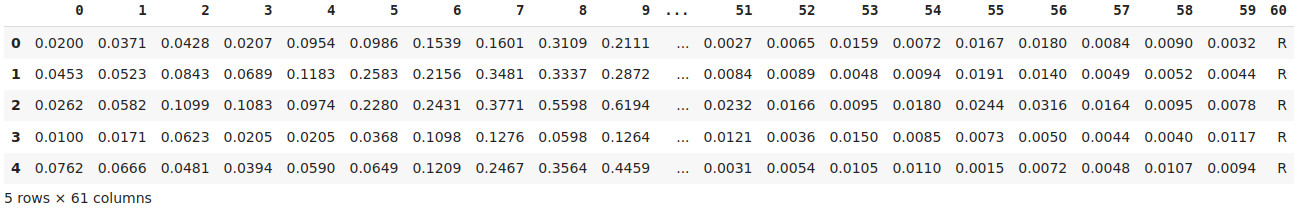
Hyperparameters evaluation methodology
We should first define a measure of how well a given set of hyperparameters is performing on our model and data.
Let's define a python function that takes as argument a set of hyperparameters, and output the expected score of our model for these hyperparameters. The expected score is computed with repeated cross validation with 5 folds and 20 repeats, and the average accuracy is returned.
from sklearn.linear_model import LogisticRegression
from sklearn.model_selection import cross_val_score
from sklearn.model_selection import RepeatedStratifiedKFold


def evaluate_hyperparameters(hyperparameters: dict) -> float:

  model = LogisticRegression(**hyperparameters)
  cv = RepeatedStratifiedKFold(n_splits=5, n_repeats=20)
  scores = cross_val_score(model, X, Y, cv=cv, scoring="accuracy", error_score=0)
  return np.mean(scores)

evaluate_hyperparameters(
    {"C": 0.1}
)0.7068176538908244Hyperparamaters optimization with optuna
Optimizing hyperparameters with optuna requires to define an objective function. The objective function defines the hyperparameters space to explore, evaluate a set of hyperparameters and return the associated score.
The hyperparameters space is defined using the inbuilt optuna methods suggest_categorical, suggest_int, suggest_float.
The hyperparameters evaluation is done using our evaluate_hyperparameters function that we defined above.
import optuna


def objective(trial):

  solver = trial.suggest_categorical("solver", ["newton-cg", "lbfgs", "liblinear"])
  penalty = trial.suggest_categorical("penalty", ["none", "l2", "l1"])
  C = trial.suggest_float("C", 1e-5, 100, log=True)

  params = {
    "solver": solver,
    "penalty": penalty,
    "C": C,
  }

  return evaluate_hyperparameters(params)
Defining the objective function is the hard work. Once it is done, we can define a study. A study is a succession of many trials, each trial being a test on a given hyperparameters combination. Notice the direction argument to indicate that the accuracy should be maximized.
Once the study is defined, the optimization process can begin. We should specificy either timeout or n_iters to specify how much computational resources we want to allocate to the optimization process.
Out of our hyperparameters space, some combinations are incompatible. These have a score of 0. The warnings from these trials are filtered out of the output.
import warnings


study = optuna.create_study(direction="maximize")

with warnings.catch_warnings():
  warnings.simplefilter("ignore")
  study.optimize(objective, timeout=120)

study.best_params
[I 2022-11-17 15:46:16,235] A new study created in memory with name: no-name-3cbaaf84-cb6f-45eb-aca4-6b9bbdf60a82
[I 2022-11-17 15:46:16,380] Trial 0 finished with value: 0.0 and parameters: {'solver': 'newton-cg', 'penalty': 'l1', 'C': 30.79640354168024}. Best is trial 0 with value: 0.0.
[I 2022-11-17 15:46:41,413] Trial 1 finished with value: 0.7406445993031359 and parameters: {'solver': 'newton-cg', 'penalty': 'none', 'C': 1.2109551238094047e-05}. Best is trial 1 with value: 0.7406445993031359.
[I 2022-11-17 15:46:41,571] Trial 2 finished with value: 0.0 and parameters: {'solver': 'liblinear', 'penalty': 'none', 'C': 0.09255479195766488}. Best is trial 1 with value: 0.7406445993031359.
[I 2022-11-17 15:46:44,381] Trial 3 finished with value: 0.5336817653890826 and parameters: {'solver': 'lbfgs', 'penalty': 'l2', 'C': 0.00012624973203480952}. Best is trial 1 with value: 0.7406445993031359.
[I 2022-11-17 15:46:49,937] Trial 4 finished with value: 0.7394367015098722 and parameters: {'solver': 'lbfgs', 'penalty': 'none', 'C': 35.66180524557645}. Best is trial 1 with value: 0.7406445993031359.
[I 2022-11-17 15:46:52,430] Trial 5 finished with value: 0.5336817653890826 and parameters: {'solver': 'newton-cg', 'penalty': 'l2', 'C': 0.0003690223936685334}. Best is trial 1 with value: 0.7406445993031359.
[I 2022-11-17 15:46:53,090] Trial 6 finished with value: 0.5346341463414636 and parameters: {'solver': 'liblinear', 'penalty': 'l2', 'C': 0.0029545040849050515}. Best is trial 1 with value: 0.7406445993031359.
[I 2022-11-17 15:46:55,174] Trial 7 finished with value: 0.7715505226480837 and parameters: {'solver': 'newton-cg', 'penalty': 'l2', 'C': 3.0775876266906406}. Best is trial 7 with value: 0.7715505226480837.
[I 2022-11-17 15:47:01,260] Trial 8 finished with value: 0.7661614401858303 and parameters: {'solver': 'lbfgs', 'penalty': 'l2', 'C': 32.39112860607594}. Best is trial 7 with value: 0.7715505226480837.
[I 2022-11-17 15:47:01,914] Trial 9 finished with value: 0.5336817653890826 and parameters: {'solver': 'liblinear', 'penalty': 'l1', 'C': 0.003616330887780869}. Best is trial 7 with value: 0.7715505226480837.
[I 2022-11-17 15:47:03,972] Trial 10 finished with value: 0.760650406504065 and parameters: {'solver': 'newton-cg', 'penalty': 'l2', 'C': 0.534881553457662}. Best is trial 7 with value: 0.7715505226480837.
[I 2022-11-17 15:47:06,251] Trial 11 finished with value: 0.7751858304297328 and parameters: {'solver': 'lbfgs', 'penalty': 'l2', 'C': 1.8458911764349824}. Best is trial 11 with value: 0.7751858304297328.
[I 2022-11-17 15:47:08,498] Trial 12 finished with value: 0.7794192799070848 and parameters: {'solver': 'lbfgs', 'penalty': 'l2', 'C': 1.137602763265833}. Best is trial 12 with value: 0.7794192799070848.
[I 2022-11-17 15:47:10,469] Trial 13 finished with value: 0.7661672473867596 and parameters: {'solver': 'lbfgs', 'penalty': 'l2', 'C': 0.4319104312673136}. Best is trial 12 with value: 0.7794192799070848.
[I 2022-11-17 15:47:12,987] Trial 14 finished with value: 0.7798025551684087 and parameters: {'solver': 'lbfgs', 'penalty': 'l2', 'C': 2.5201402079578057}. Best is trial 14 with value: 0.7798025551684087.
[I 2022-11-17 15:47:13,161] Trial 15 finished with value: 0.0 and parameters: {'solver': 'lbfgs', 'penalty': 'l1', 'C': 0.039511772550540024}. Best is trial 14 with value: 0.7798025551684087.
[I 2022-11-17 15:47:15,692] Trial 16 finished with value: 0.777979094076655 and parameters: {'solver': 'lbfgs', 'penalty': 'l2', 'C': 2.732619752896652}. Best is trial 14 with value: 0.7798025551684087.
[I 2022-11-17 15:47:17,473] Trial 17 finished with value: 0.731521486643438 and parameters: {'solver': 'lbfgs', 'penalty': 'l2', 'C': 0.191913503158126}. Best is trial 14 with value: 0.7798025551684087.
[I 2022-11-17 15:47:17,640] Trial 18 finished with value: 0.0 and parameters: {'solver': 'lbfgs', 'penalty': 'l1', 'C': 7.81783345490552}. Best is trial 14 with value: 0.7798025551684087.
[I 2022-11-17 15:47:22,125] Trial 19 finished with value: 0.7364459930313589 and parameters: {'solver': 'lbfgs', 'penalty': 'none', 'C': 0.0032920655428724617}. Best is trial 14 with value: 0.7798025551684087.
[I 2022-11-17 15:47:22,821] Trial 20 finished with value: 0.6428106852497097 and parameters: {'solver': 'liblinear', 'penalty': 'l2', 'C': 0.026122896936888677}. Best is trial 14 with value: 0.7798025551684087.
[I 2022-11-17 15:47:25,962] Trial 21 finished with value: 0.7749361207897791 and parameters: {'solver': 'lbfgs', 'penalty': 'l2', 'C': 5.7940414471240365}. Best is trial 14 with value: 0.7798025551684087.
[I 2022-11-17 15:47:28,871] Trial 22 finished with value: 0.7773867595818815 and parameters: {'solver': 'lbfgs', 'penalty': 'l2', 'C': 1.4190916430533451}. Best is trial 14 with value: 0.7798025551684087.
[I 2022-11-17 15:47:34,494] Trial 23 finished with value: 0.7597212543554008 and parameters: {'solver': 'lbfgs', 'penalty': 'l2', 'C': 77.4189956654296}. Best is trial 14 with value: 0.7798025551684087.
[I 2022-11-17 15:47:37,737] Trial 24 finished with value: 0.7747386759581881 and parameters: {'solver': 'lbfgs', 'penalty': 'l2', 'C': 8.787780937476255}. Best is trial 14 with value: 0.7798025551684087.
[I 2022-11-17 15:47:39,806] Trial 25 finished with value: 0.7689605110336818 and parameters: {'solver': 'lbfgs', 'penalty': 'l2', 'C': 0.6658125540440398}. Best is trial 14 with value: 0.7798025551684087.
[I 2022-11-17 15:47:41,512] Trial 26 finished with value: 0.7112659698025552 and parameters: {'solver': 'lbfgs', 'penalty': 'l2', 'C': 0.14015439489249706}. Best is trial 14 with value: 0.7798025551684087.
[I 2022-11-17 15:47:42,934] Trial 27 finished with value: 0.6163124274099884 and parameters: {'solver': 'lbfgs', 'penalty': 'l2', 'C': 0.015376354429056431}. Best is trial 14 with value: 0.7798025551684087.
[I 2022-11-17 15:47:47,623] Trial 28 finished with value: 0.7287862950058072 and parameters: {'solver': 'lbfgs', 'penalty': 'none', 'C': 12.967005248040023}. Best is trial 14 with value: 0.7798025551684087.
[I 2022-11-17 15:47:48,742] Trial 29 finished with value: 0.7625900116144018 and parameters: {'solver': 'liblinear', 'penalty': 'l1', 'C': 1.277466983339063}. Best is trial 14 with value: 0.7798025551684087.
[I 2022-11-17 15:47:48,869] Trial 30 finished with value: 0.0 and parameters: {'solver': 'newton-cg', 'penalty': 'l1', 'C': 3.46171570204636}. Best is trial 14 with value: 0.7798025551684087.
[I 2022-11-17 15:47:51,787] Trial 31 finished with value: 0.779047619047619 and parameters: {'solver': 'lbfgs', 'penalty': 'l2', 'C': 0.86154741970487}. Best is trial 14 with value: 0.7798025551684087.
[I 2022-11-17 15:47:54,207] Trial 32 finished with value: 0.7388966318234611 and parameters: {'solver': 'lbfgs', 'penalty': 'l2', 'C': 0.2509880331902386}. Best is trial 14 with value: 0.7798025551684087.
[I 2022-11-17 15:48:00,511] Trial 33 finished with value: 0.7701045296167248 and parameters: {'solver': 'lbfgs', 'penalty': 'l2', 'C': 17.024171904597186}. Best is trial 14 with value: 0.7798025551684087.
[I 2022-11-17 15:48:02,705] Trial 34 finished with value: 0.7745528455284554 and parameters: {'solver': 'lbfgs', 'penalty': 'l2', 'C': 1.1357683240229643}. Best is trial 14 with value: 0.7798025551684087.
[I 2022-11-17 15:48:07,230] Trial 35 finished with value: 0.7305342624854819 and parameters: {'solver': 'lbfgs', 'penalty': 'none', 'C': 74.66515628654487}. Best is trial 14 with value: 0.7798025551684087.
[I 2022-11-17 15:48:09,766] Trial 36 finished with value: 0.6972241579558652 and parameters: {'solver': 'newton-cg', 'penalty': 'l2', 'C': 0.09275954032613976}. Best is trial 14 with value: 0.7798025551684087.
[I 2022-11-17 15:48:16,272] Trial 37 finished with value: 0.7388675958188153 and parameters: {'solver': 'lbfgs', 'penalty': 'none', 'C': 2.2139799541091597e-05}. Best is trial 14 with value: 0.7798025551684087.
{'solver': 'lbfgs', 'penalty': 'l2', 'C': 2.5201402079578057}
Inbuilt vizualisations
Optuna provides inbuilt vizualisations on study object that may give a better comprehension on the optimization process.
from optuna.visualization import plot_optimization_history

plot_optimization_history(study)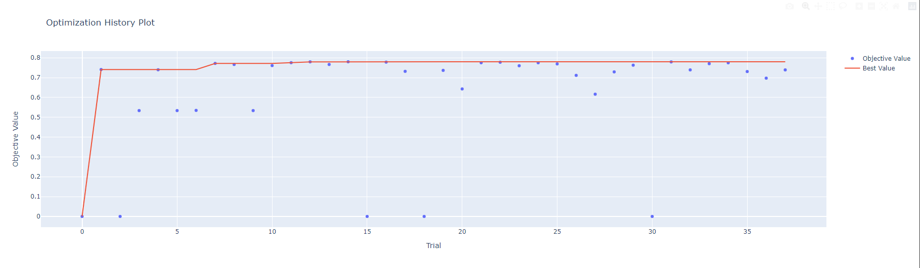
from optuna.visualization import plot_parallel_coordinate

plot_parallel_coordinate(study)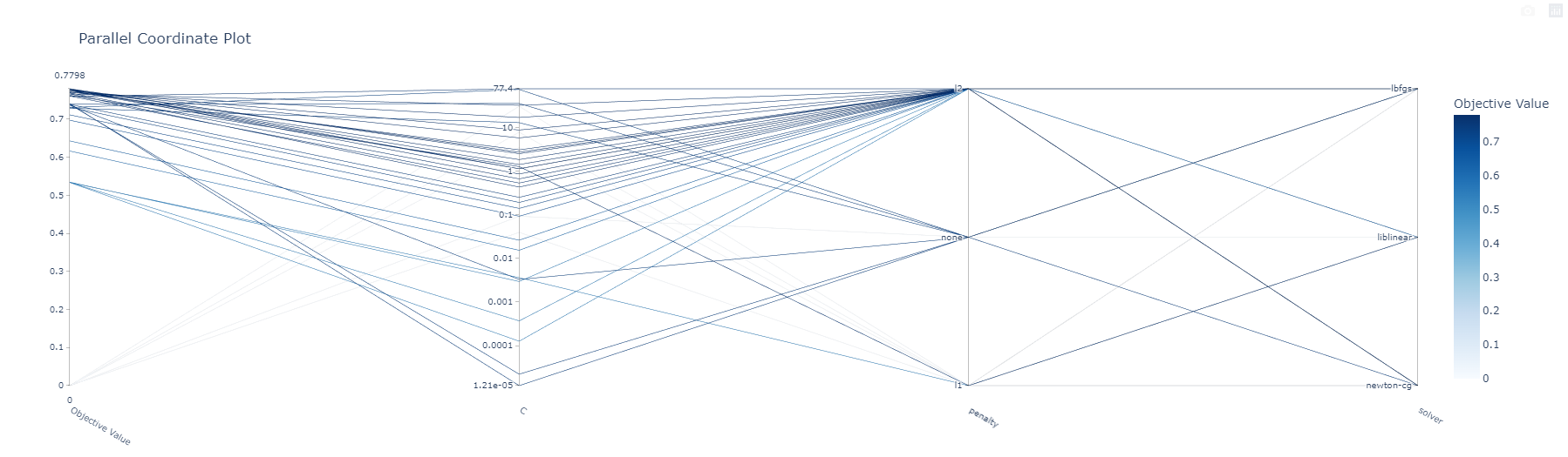
Further reading and ending thoughts
Bayesian optimization provides a simple yet elegant approach to one part of the machine learning process. It provides the advantages of an automated method (integration in MLops pipeline, repeatability, maintanability, etc.) while being far more resource and time efficient than its most used counterparts: random and grid search.
The ability to put machine learning models in production with the quality standards that match the software development world has been the main painpoint since the emergence of machine learning. Automating tasks that used to be done manually, like hyperparameters optimization, is crucial to improve the most challenging task in machine learning: putting high quality, maintainable machine learning-based software in production.
For further reading on bayesian optimization, I recommend this excellent blog article.
For a simple implementation of random search or grid search on the same dataset, I recommend reading this machine learning mastery blog post